Generating elementary cellular automata with Python

Cellular automata (CA) are discrete models defined by a board and transition function. In the simplest case, a board is an array where cells can take on values ‘0’ or ‘1’ and a transition function is a method that describes how the values of each cell on the board changes from one time step to the next. Specifically, the transition function will take the value of a cell and its two neighbors as input, and output the value of that cell at the next point in time. An example of a (boring) transition function is, “if the neighors of a cell are both ‘1’ at time t, then the cell will take the value ‘1’ at time t+1, else it will take the value ‘0’”. The transition function is applied to all cells on a board at the same time in order to move from one time step to the next.

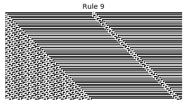
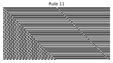
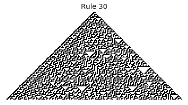
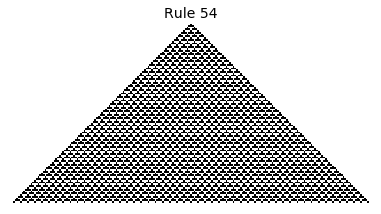
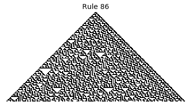
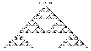
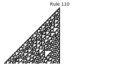
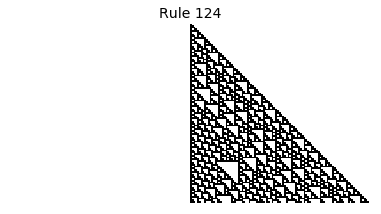
If, as above, we simply consider 1D boards, cells with binary values, and transition functions that operate as a function of a cell and its immediate neighbor’s values, then there are only 256 possible transition functions. These are called elementary cellular automata. Despite the simplicity of these rules, there exist elementary cellular automata that exhibit complex behavior - so much so that they are the main topic in Stephen Wolfram’s 1200 page book “A New Kind of Science”. Some of the elementary CA rules have actually been shown to be capable of universal computation (that is, with carefully designed input boards, or initial states, you can perform arbitrary computations by just iterating according to one of the elementary cellular automata transition functions).

Science, new or old, aside, this blog post is simply about simulating the elementary cellular automata using Python. This is a fun excersise that results in some pretty cool looking pictures, but, more importantly, that demonstrates the wide range of possible extensions that can be explored (e.g. the reader can consider: can this be done in 2D, can this be done faster, what all can be computed with CA, can this be done in color, etc.).

The code

The following code can be run cell by cell in a Jupyter notebook. We start by doing some magic and importing the usual packages.

%matplotlib inline
import numpy as np
import matplotlib.pyplot as plt

First, we implement the elementary CA transition functions as lookup tables. These simply map the possible combinations of the states a cell and its two neighbors to the next value of the cellv. See here for more information about the mappings (i.e. what the rule idx defined below means).

def get_rule(idx):
    if idx < 256:
        input_patterns = [
            (1,1,1),
            (1,1,0),
            (1,0,1),
            (1,0,0),
            (0,1,1),
            (0,1,0),
            (0,0,1),
            (0,0,0)
        ]
        outputs = list(map(int,format(idx, "#010b")[2:]))
        mapping = dict(zip(input_patterns, outputs))
        mapping["name"] = "Rule %d" % (idx)
        return mapping
    else:
        raise ValueError("Rule number out of range")

This method will perform one step on a given board according to a given rule. It assumes zero padding on the board’s boundaries.

def iterate(board, rule):
    board = np.pad(board, (1, 1), 'constant', constant_values=(0,0))
    new_board = np.zeros_like(board)
    for i in range(1, board.shape[0] - 1):
        new_board[i] = rule[tuple(board[i-1:i+2])]
    return new_board[1:-1]

Now that we have expressed rules and given a method to use a rule to move from one state to the next, we can make a helper function that wraps up the task of “permorming many iterations” nicely. With elementary cellular automata, the information in an initial state can only propagate outwards at a rate of 1 cell per iteration, therefore this method pads the intial configuration with num_iterations zeros on each side of the intial_board. This garuntees that our CA will have enough space to grow throughout the last iteration. The method will return an array of size (num_iterations + 1, len(initial_board) + 2*num_iterations) where each row, i, is the output of the CA at timestep i.

def generate_map(initial_board, rule, num_iterations=100):
    
    if isinstance(initial_board, list):
        board = np.array(initial_board)
    else:
        board = initial_board
    
    board = np.pad(board, (num_iterations, num_iterations), 'constant', constant_values=(0,0))
    
    rows = [board]
    for i in range(num_iterations):
        board = iterate(board, rule)
        rows.append(board)

    rows = np.array(rows)
    return rows

Finally, we create a simple method for visualizing the output of generate_map.

def visualize_board(board, title=None):
    plt.figure(figsize=(5,2.5))
    plt.imshow(board, cmap="Greys")
    plt.axis("off")
    if title is not None:
        plt.title(title, fontsize=14)
    plt.show()
    plt.close()

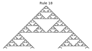
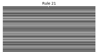
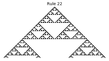
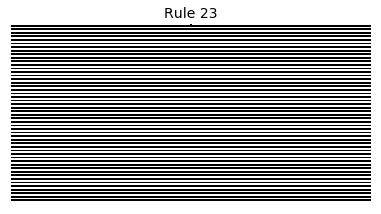
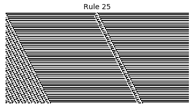
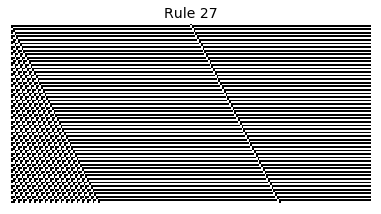
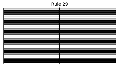
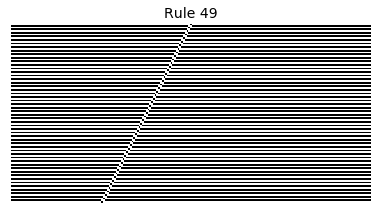
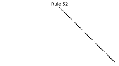
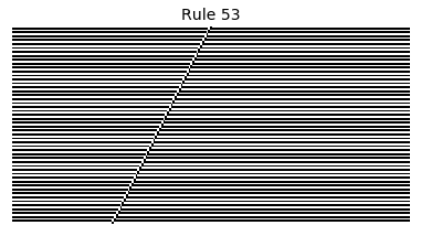
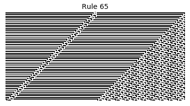
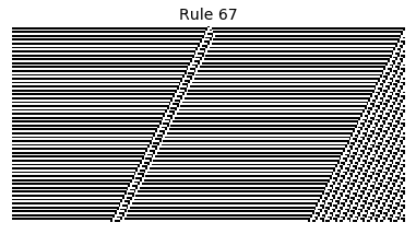
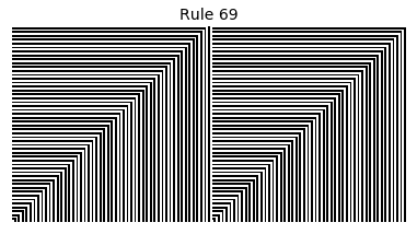
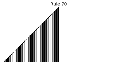
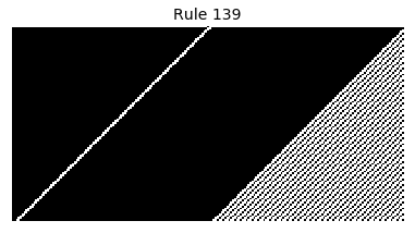
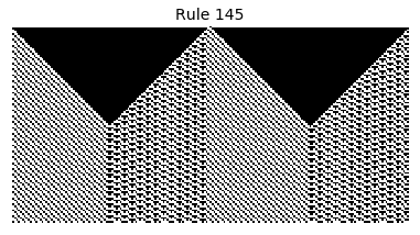
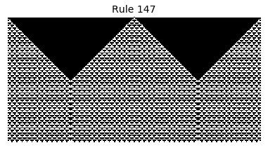
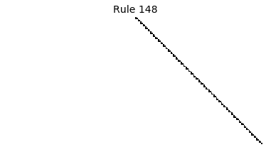
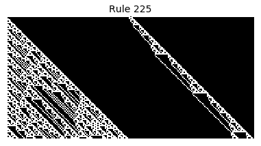
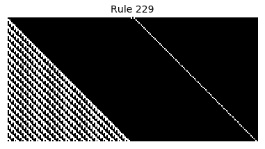
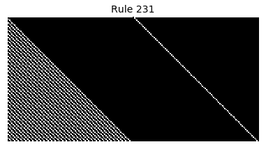
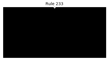
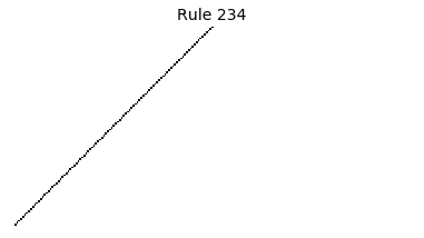
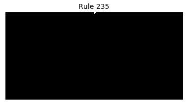
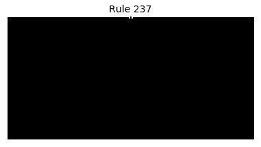
The results

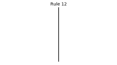
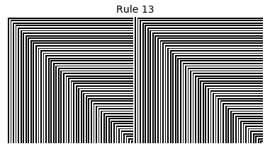
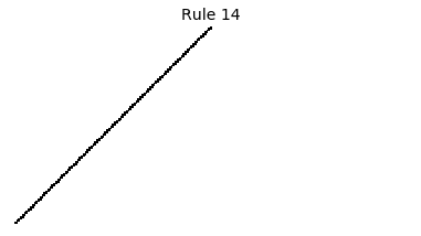
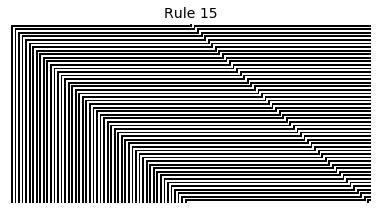
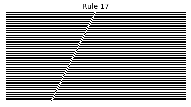
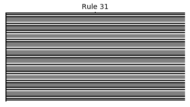
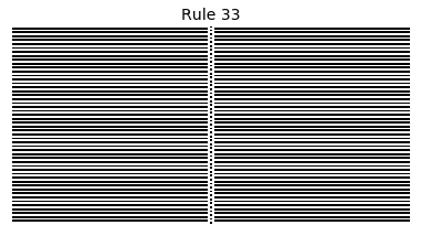
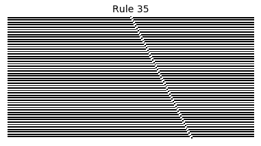
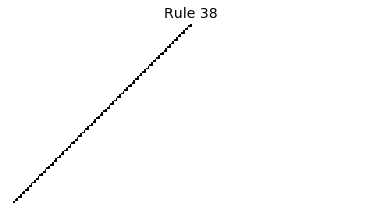
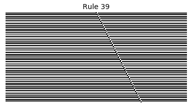
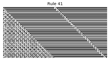
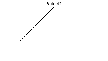
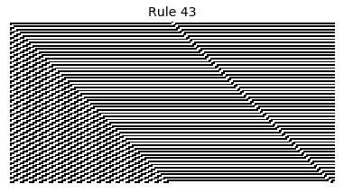
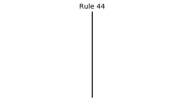
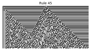
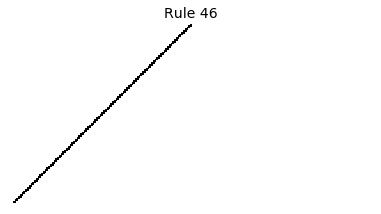
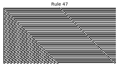
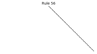
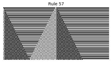
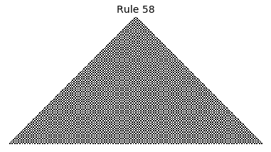
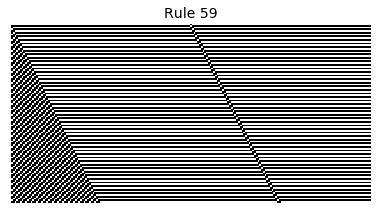
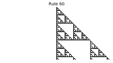
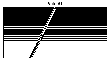
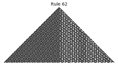
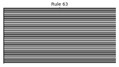
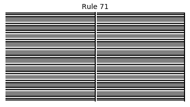
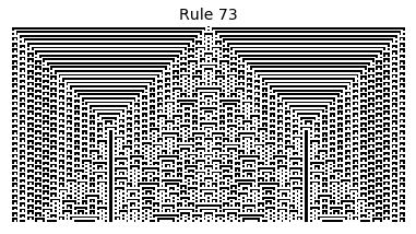
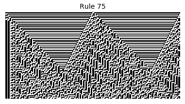
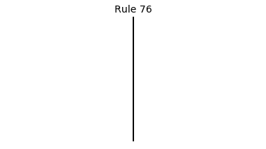
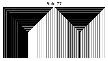
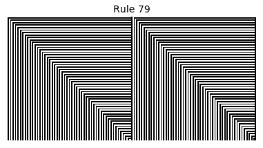
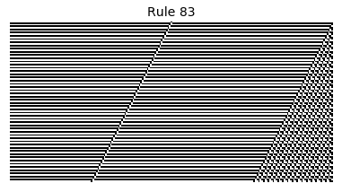
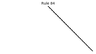
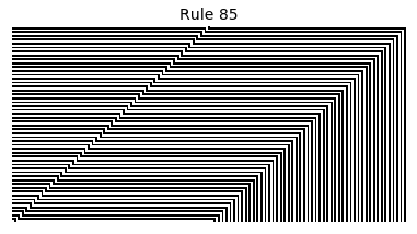
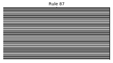
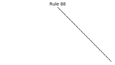
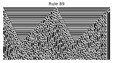
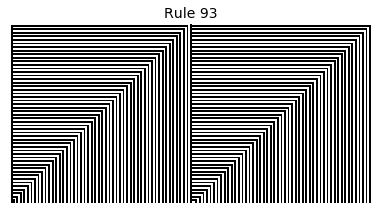
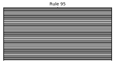
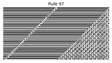
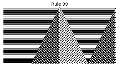
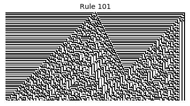
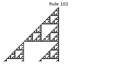
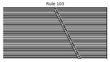
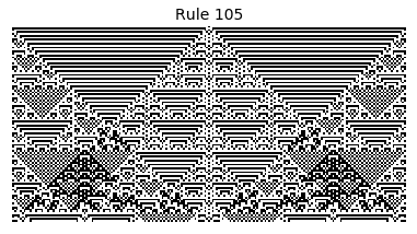
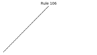
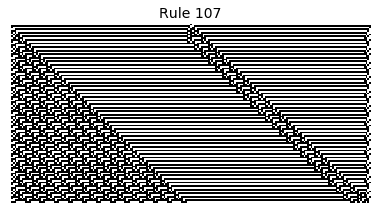
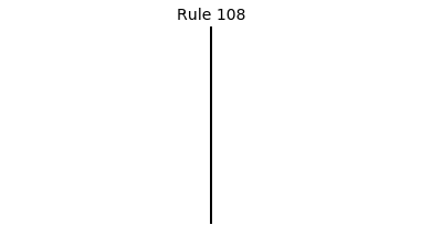
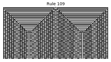
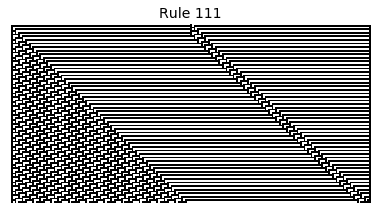
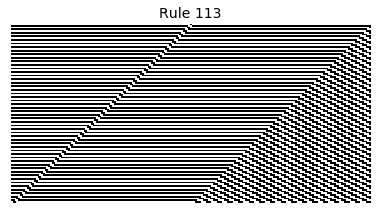
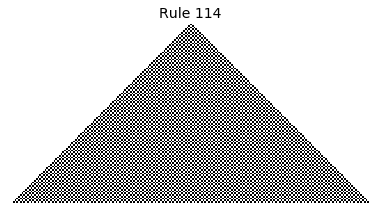
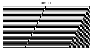
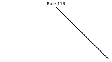
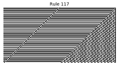
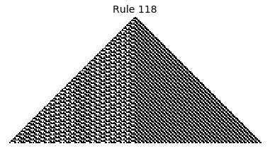
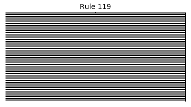
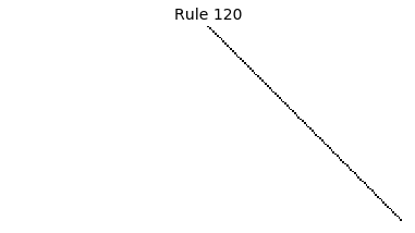
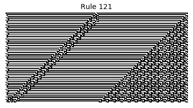
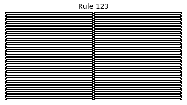
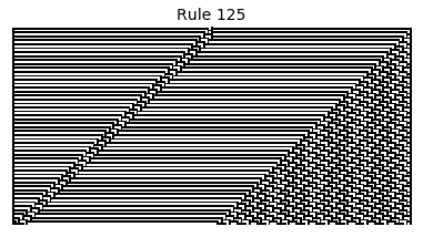
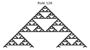
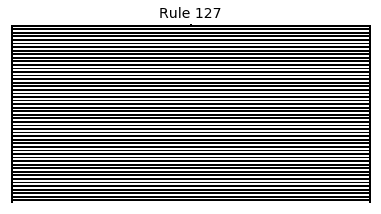
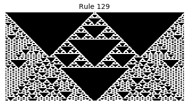
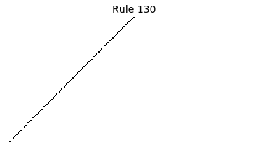
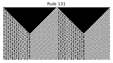
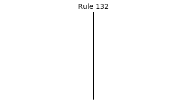
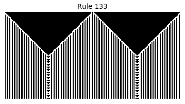
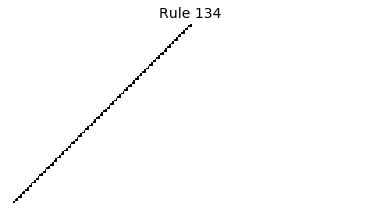
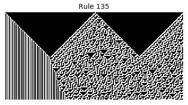
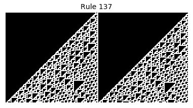
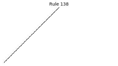
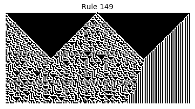
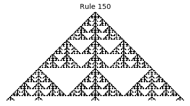
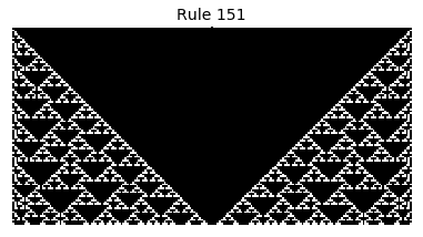
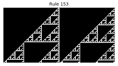
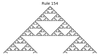
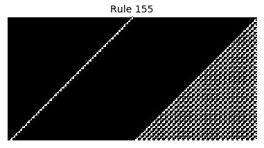
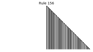
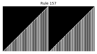
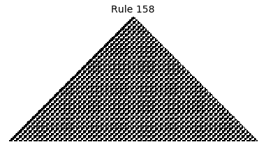
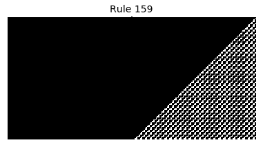
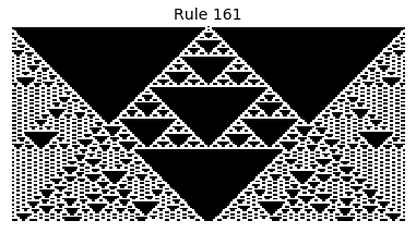
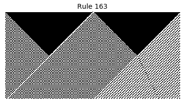
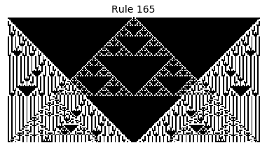
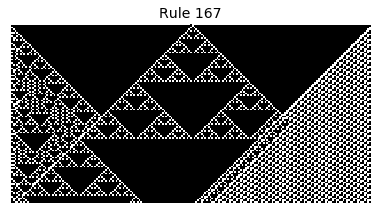
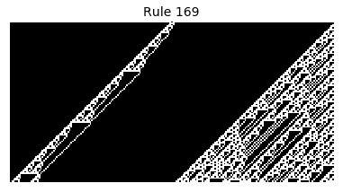
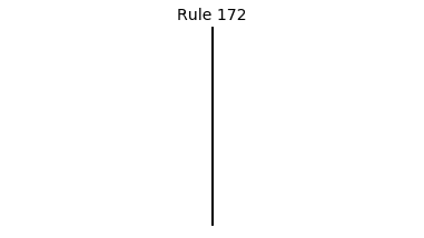
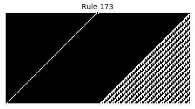
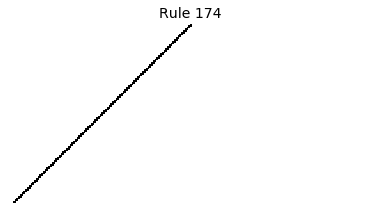
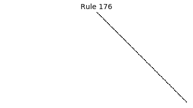
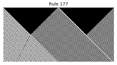
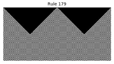
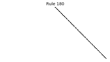
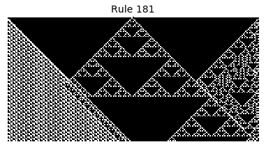
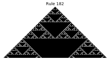
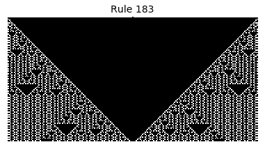
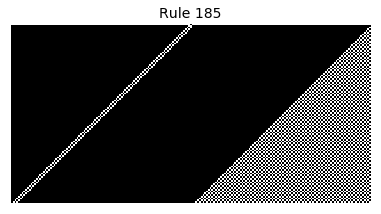
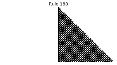
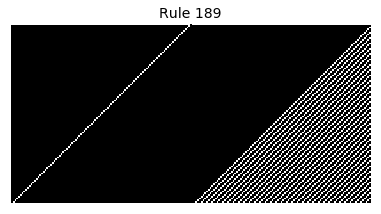
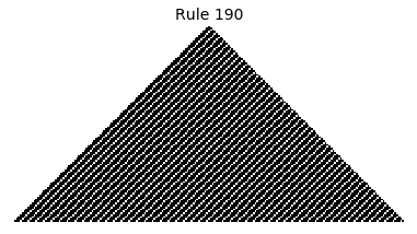
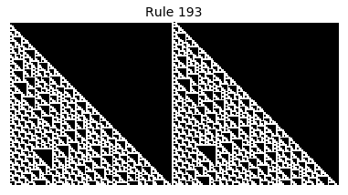
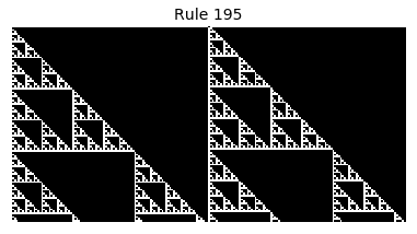
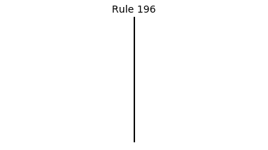
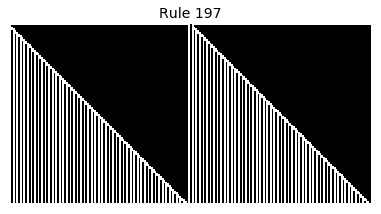
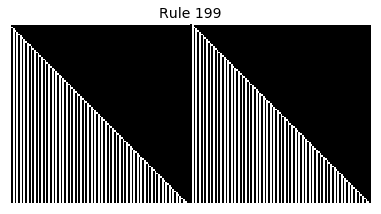
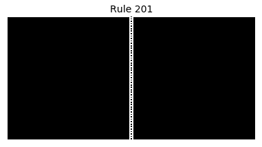
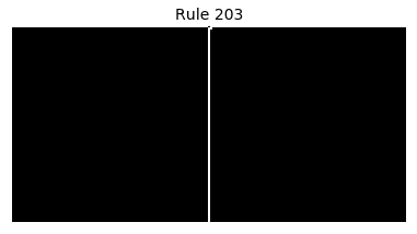
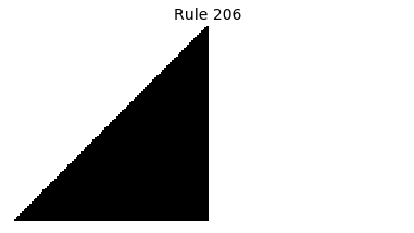
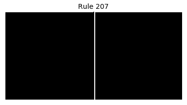
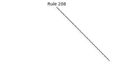
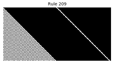
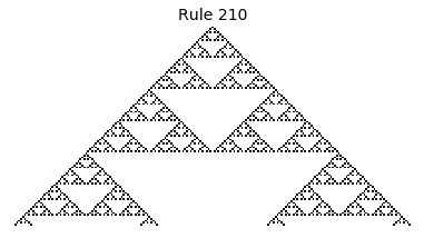
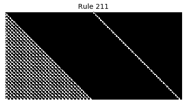
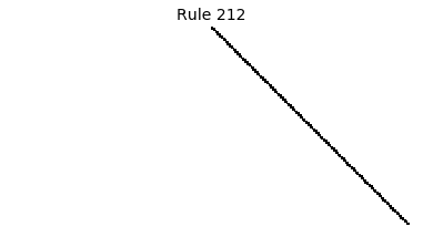
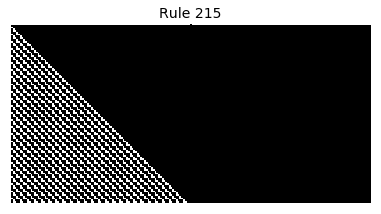
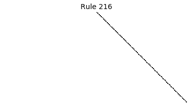
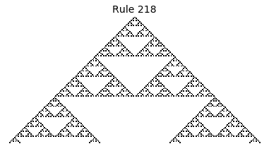
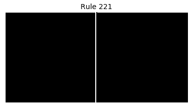
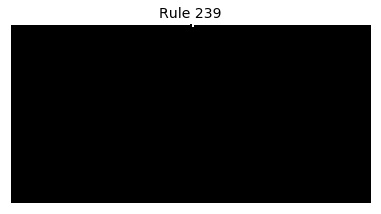
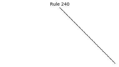
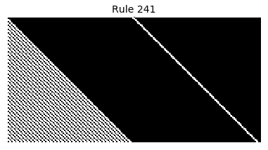
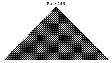
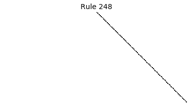
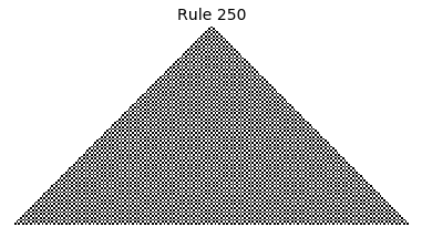
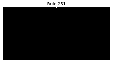
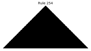
Now that we have all the pieces, we can easily simulate the first 100 iterations of each of the 256 elementary cellular automata.

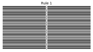
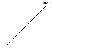
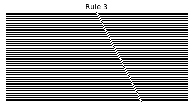
for i in range(256):
    rule = get_rule(i)
    board = generate_map([0,1,0], rule, num_iterations=100)
    visualize_board(board, rule["name"])